




Transmission distance is not a property of the cable alone. It is the result of a system budget: the fiber you install, the data rate you run over it, the wavelength your transceivers use, the loss your connectors and splices add, and the dispersion the signal accumulates on the way. Change any one of these and the maximum distance changes with it.
That is why two links built with identical cable can behave completely differently - one runs 40 km without an error, the other fails at 300 m. This guide explains which variables set the ceiling, how to calculate the ceiling for your own link, and what to check when a link falls short of its rated reach.

Distance Is a Link Budget, Not a Cable Spec
Before looking at individual factors, it helps to know how the pieces rank. For a normally designed link, maximum distance is decided in roughly this order:
- Fiber type and grade - single-mode or multimode, and which category within each
- Data rate and optical interface standard - 1G, 10G, 100G, 400G behave very differently on the same fiber
- Transceiver specification - launch power, receiver sensitivity, rated reach
- Total link loss - fiber attenuation plus every connector, splice and splitter in the path
- Dispersion - modal dispersion on multimode, chromatic dispersion on long single-mode spans
- Environment and installation quality - mostly a reliability and margin issue, not a first-order distance limit
Environmental conditions belong on this list, but not at the top. Temperature, moisture and mechanical stress mainly erode your margin and long-term reliability. They rarely decide whether a correctly designed link reaches 10 km or 40 km.
Fiber Type and Modal Bandwidth
Single-mode fiber carries one propagation mode, so it avoids modal dispersion entirely and is the only realistic choice beyond a few hundred metres. Multimode fiber carries many modes that arrive at slightly different times, and that spreading - not attenuation - is what caps its reach at high data rates.
This is why multimode is specified by effective modal bandwidth rather than by distance. OM3 is rated at 2000 MHz·km at 850 nm and OM4 at 4700 MHz·km; the higher figure is exactly why OM4 fiber supports longer 10G and 100G channels than OM3 on otherwise identical hardware. If you are still deciding between the two families, the trade-offs in cost, transceiver price and upgrade headroom are covered in this single-mode versus multimode comparison.
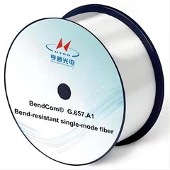
Within single-mode, the category matters less for raw distance than people assume. G.652.D fiber is the mainstream choice, specified in ITU-T Recommendation G.652 with cabled attenuation of no more than 0.4 dB/km at 1310 nm and 0.3 dB/km at 1550 nm. Bend-insensitive G.657 grades, defined in ITU-T G.657, do not transmit further in a straight span - they simply lose less where the route forces tight bends.
So what actually happens if you pick the wrong fiber? Rarely a clean "distance shortfall". More often it is one of these: the transceiver will not link at all because a single-mode module cannot couple properly into a 50 µm core; the link comes up but errors under load because modal bandwidth is insufficient for the rate; or the receiver is overloaded because the span is far shorter than the module was designed for.
Data Rate, Wavelength and Dispersion
The same fiber supports very different distances depending on what you run over it. Higher symbol rates mean shorter bit periods, so a given amount of pulse spreading consumes a larger fraction of the eye. The result is the pattern every network engineer eventually notices: reach falls as rate rises.
| Optical interface | Fiber | Wavelength | Maximum reach (IEEE 802.3) |
|---|---|---|---|
| 1000BASE-SX | OM3 | 850 nm | 550 m |
| 10GBASE-SR | OM3 / OM4 | 850 nm | 300 m / 400 m |
| 100GBASE-SR4 | OM3 / OM4 | 850 nm | 70 m / 100 m |
| 10GBASE-LR | Single-mode | 1310 nm | 10 km |
| 10GBASE-ER | Single-mode | 1550 nm | 40 km |
| 100GBASE-LR4 | Single-mode | 1310 nm | 10 km |
| 100GBASE-ER4 | Single-mode | 1550 nm | 40 km |

Note that OM4 buys you 100 m at 10G but only 30 m at 100G. Fiber grade cannot compensate indefinitely for rate.
Wavelength works in two directions at once. At 1550 nm attenuation is lowest - typically around 0.19–0.21 dB/km on G.652.D against 0.32–0.35 dB/km at 1310 nm - which is why long-haul and DWDM systems live in the C-band. But 1550 nm is also where standard single-mode fiber shows roughly 17 ps/nm·km of chromatic dispersion, while 1310 nm sits near the zero-dispersion point. On a 10G or 25G link past about 60–80 km, dispersion, not power, becomes the binding constraint, and you need compensation or a coherent interface rather than a hotter transmitter.
Optical Power Budget
This is the calculation that turns the discussion above into a number. Start with what the transceiver gives you:
Available power budget (dB) = minimum transmitter output power (dBm) − receiver sensitivity (dBm)
Then subtract everything the link consumes:
- Fiber attenuation: attenuation coefficient (dB/km) × length (km)
- Connector loss: number of mated pairs × loss per pair (typically 0.2–0.5 dB in the field; TIA allows up to 0.75 dB)
- Splice loss: number of fusion splices × loss per splice (typically under 0.1 dB, with 0.3 dB a common acceptance limit)
- Passive component loss: PON splitters, patch panels, WDM filters
- System margin: 3 dB is the conventional allowance for ageing, repairs and measurement uncertainty
A worked example for a 10 km single-mode link at 1310 nm, using representative datasheet values - always substitute the figures from your own module datasheet:
- Transmitter minimum output: −8.0 dBm; receiver sensitivity: −18.0 dBm → budget 10.0 dB
- Fiber: 10 km × 0.36 dB/km = 3.6 dB
- Connectors: 4 mated pairs × 0.5 dB = 2.0 dB
- Splices: 2 × 0.1 dB = 0.2 dB
- Total link loss = 5.8 dB; remaining margin = 4.2 dB
Above 3 dB of margin, the link is sound. Below it, you are one dirty connector or one repair splice away from errors. And if the calculation passes but the link still fails, the limit is not power - look at dispersion or at a rate/interface mismatch.
Connectors, Splices and Bending
In a laboratory the fiber dominates the loss budget. In the field, the discrete events usually do. Four connector pairs at 0.5 dB each cost the same as 5.5 km of G.652.D fiber at 1310 nm - and connector count is the variable most often underestimated at the design stage.
Three failure modes account for most of the shortfall between calculated and measured loss:
- Contaminated end faces. A single particle on a ferrule can add anything from a fraction of a dB to complete link failure, and it is the first thing to inspect on any link that degraded without a physical change.
- Poor fusion splices. Core misalignment, cleave angle errors and contamination all show up as elevated splice loss. A splice consistently above 0.3 dB should be re-made rather than accepted.
- Bending. Macrobending - a cable pulled around a tray corner tighter than its minimum bend radius - appears as a localised step on an OTDR trace and is strongly wavelength-dependent, worse at 1550 nm than at 1310 nm. Microbending from crushing or over-tight cable ties is more diffuse and harder to localise. The bending loss behaviour of G.657 fiber is what makes it worth specifying for in-building and FTTH routes where installers cannot guarantee generous radii.
Transceiver Reach and Compatibility
The distance printed on an optical module is a system rating derived from the interface standard, not a promise about your particular route. It assumes a specific fiber type, a specific wavelength, and a channel insertion loss the standard defines. Three checks before you commit:
- Fiber type and wavelength must match on both ends. An 850 nm module and a single-mode span are simply incompatible, and a 1310 nm module will not interoperate with a 1550 nm one.
- Your calculated link loss must sit below the interface's channel insertion loss allowance, which is specified per PHY type by the IEEE 802.3 Working Group.
- Check the receiver overload point, not just sensitivity. Putting a 40 km ER module on a 500 m link can saturate the receiver and produce errors that look exactly like excessive loss. Fit an attenuator.
For procurement, the practical rule is to ask suppliers for the three numbers that let you verify the claim yourself: minimum transmitter output power, receiver sensitivity, and rated channel insertion loss. A quoted "20 km module" without those figures cannot be checked against your route.
Environmental and Installation Conditions
Environment affects distance indirectly, by eating margin and by degrading the cable over time. Outdoor cables need water-blocking, UV-resistant and mechanically robust structures because moisture ingress into a damaged sheath or splice closure, and crush loading that induces microbending, are what push a link out of budget years after commissioning. Cyclic temperature extremes matter mainly at the boundaries of the specified operating range and through long-term ageing, not as a day-to-day distance variable.
One correction worth making explicitly, because it appears constantly in cable literature: flame-retardant and fire-resistant ratings do not extend transmission distance. They exist to satisfy building fire codes, limit flame spread and control smoke and halogen emission. Flexibility and bend performance genuinely affect installed loss; flame rating does not. Specify both, but do not confuse the two.
Frequently Asked Questions
How far can single-mode fiber actually transmit?
It depends on the interface, not the fiber. Standard Ethernet interfaces on single-mode span 10 km (LR), 40 km (ER) and 80 km (ZR-class, vendor-specified). With amplification and dispersion compensation, submarine and long-haul systems run thousands of kilometres over the same fiber category. The fiber is almost never the limiting element.
Why does the same fiber support less distance at higher data rates?
Two reasons. Higher rates shorten the bit period, so a fixed amount of pulse spreading from dispersion consumes proportionally more of the eye. And higher-rate receivers generally need more optical power for the same error rate, which shrinks the power budget. Both effects push in the same direction.
Is 1310 nm or 1550 nm better for long distance?
1550 nm has lower attenuation, so it wins on power budget over long spans. But 1310 nm sits near the zero-dispersion wavelength of standard single-mode fiber, so it is more tolerant on high-rate links. For a loss-limited span, choose 1550 nm; for a dispersion-limited one, 1310 nm or an interface with dispersion compensation.
My link is well within the module's rated distance but still errors. Why?
The most common causes, in order: contaminated connector end faces, more connector pairs in the path than the budget assumed, a high-loss splice, a bend violating minimum radius, or receiver overload on a short link with a long-reach module. Measure the loss first - it separates power problems from everything else.
Do low-loss or "premium" cables extend distance meaningfully?
Sometimes, but the effect is bounded and needs to be quantified. Moving from 0.35 dB/km to 0.19 dB/km at 1550 nm saves 1.6 dB over 10 km - real, but smaller than three sloppy connectors. Ultra-low-loss fiber earns its price on long unrepeatered spans, not on campus links. Always ask which wavelength a quoted attenuation figure refers to, and remember that the transceiver's rated reach still caps the link regardless of how good the fiber is.
Summary
Fiber optic transmission distance is set by a system, not by a cable. Fix the data rate and interface standard first, then the fiber type and grade, then calculate the power budget against your real connector and splice count, and finally check dispersion for long or high-rate spans. Treat environmental specification as a reliability and margin decision - necessary, but a different question from reach.
If you are specifying cable for a route with a known length and rate, the useful next step is to work backwards: take the interface's channel insertion loss allowance, subtract 3 dB of margin, subtract your connector and splice budget, and see what attenuation coefficient the remaining figure demands of the fiber. That number, not a marketing distance, is what should drive the specification.